Computing LLPR uncertainties

This tutorial demonstrates how to train a model with uncertainties using metatrain. It involves the computation of the uncertainties on ethanol molecules, using the last-layer prediction rigidity (LLPR) approximation. Both total and local (LPR) uncertainties are computed

The baseline model was trained using the following training options, where the training set consists of 100 structures from the QM9 dataset.

device: cpu
base_precision: 64
seed: 42

architecture:
  name: soap_bpnn
  training:
    batch_size: 10
    num_epochs: 10
    learning_rate: 0.01

# Section defining the parameters for system and target data
training_set:
  systems: qm9_reduced_100.xyz
  targets:
    energy:
      key: U0
      unit: hartree  # very important to run simulations

validation_set: 0.1
test_set: 0.0

Once a model is trained, you can add LLPR uncertainties to it by launching a training run with the “llpr” architecture, on the same data. In this case, the training options to add LLPR uncertainties are as follows:

device: cpu
base_precision: 64
seed: 42

architecture:
  name: llpr
  training:
    model_checkpoint: model.ckpt
    batch_size: 4

# Section defining the parameters for system and target data
training_set:
  systems: qm9_reduced_100.xyz
  targets:
    energy:
      key: U0
      unit: hartree  # very important to run simulations

validation_set: 0.1
test_set: 0.0

Adding LLPR uncertainties is very cheap compared to training a model, as it only involves one pass through the training data (equivalent to one epoch of training).

You can repeat the same training yourself with

#!/bin/bash

mtt train options.yaml -o model.pt
mtt train options-llpr.yaml -o model-llpr.pt

A detailed step-by-step introduction on how to train a model is provided in the Basic Usage tutorial.

As an example, we will compute the energies and uncertainties of the LLPR model on a few ethanol structures.

import ase.io
import matplotlib.pyplot as plt
from ase.visualize.plot import plot_atoms
from matplotlib.colors import LogNorm
from metatomic.torch import ModelOutput
from metatomic.torch.ase_calculator import MetatomicCalculator


# load 5 ethanol structures
structures = ase.io.read("ethanol_reduced_100.xyz", ":5")

# load the model as an ASE calculator
calc = MetatomicCalculator(
    "model-llpr.pt", extensions_directory="extensions/", device="cpu"
)

# the uncertainties are available throguh the ``run_model`` method of the calculator
predictions = calc.run_model(
    structures,
    {
        "energy": ModelOutput(per_atom=False),
        "energy_uncertainty": ModelOutput(per_atom=False),
    },
)

# print the energies and uncertainties

energies = predictions["energy"].block().values.squeeze().numpy()
uncertainties = predictions["energy_uncertainty"].block().values.squeeze().numpy()

print(energies)
print(uncertainties)

[-154.97815979 -154.97894444 -154.97760901 -154.9749007  -154.97667892]
[0.00248884 0.00265013 0.00304968 0.00230806 0.0019654 ]

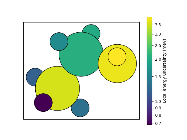
We can also obtain per-atom uncertainties (local prediction rigidity, LPR). As an example, we will compute the uncertainties on an ethanol structure.

structure = structures[0]
predictions = calc.run_model(
    structure,
    {
        # here, we use per_atom=True to request per-atom uncertainties
        "energy_uncertainty": ModelOutput(per_atom=True),
    },
)
local_uncertainty = predictions["energy_uncertainty"].block().values.squeeze().numpy()
local_uncertainty = local_uncertainty * 1000.0  # convert from eV to meV

norm = LogNorm(vmin=min(local_uncertainty), vmax=max(local_uncertainty))
colormap = plt.get_cmap("viridis")
colors = colormap(norm(local_uncertainty))
ax = plot_atoms(structure, colors=colors, rotation="180x,0y,0z")
custom_ticks = [0.7, 0.8, 0.9, 1.0, 1.5, 2.0, 2.5, 3.0, 3.5]
cbar = plt.colorbar(
    plt.cm.ScalarMappable(norm=norm, cmap=colormap),
    ax=ax,
    label="Local energy uncertainty (meV)",
    ticks=custom_ticks,
)
cbar.ax.set_yticklabels([f"{tick}" for tick in custom_ticks])
cbar.minorticks_off()
ax.set_xticks([])
ax.set_yticks([])
plt.show()